
Internet usage has been accelerated by the pandemic. All of those activities on the internet eventually become requests or workloads on servers, applications, and systems. Scalability becomes a challenge. In the previous article, you learned how streaming, pipelining, and parallelization help your applications maximize the utilization of your resources. In this article, we will discuss the strategies and considerations for implementing high-throughput applications.
Implement streaming
Ensure data consistency when breaking down a task
Streaming breaks a big task into smaller chunks and processes them in sequence. In this context, ensuring data consistency, or atomicity, can have several meanings.
First, it means the atomicity of the original task. Breaking down the task does not change the task when we put the smaller slices back together. For example, if we break the “copy-paste 1 TB file” tasks into 33 million smaller tasks, each task copies and pastes 32 KB of the file and processes it separately. After the processing, the 33 million tasks will be consolidated into a 1 TB file.
Second, it means the atomicity of each smaller task. It either fully and successfully commits or completely fails. We will discuss how to achieve the atomicity of each smaller task in a later section. For now, we assume that the smaller tasks are already atomic.
If our big job can be broken down to many smaller tasks, when every small task finishes, the big job is done. This is the best situation: we have a perfect breakdown that is exactly equal to the original.
Unfortunately, it’s not easy to ensure that each small task is done just once. The most common situation is “false failure”: a small task finishes, but fails to mark down or tell others it succeeded. Therefore, this task is mistakenly considered “failed.” False failures are an especially big problem when our job is running in a complicated environment. These failures can include machine failure, network failure, and process failure.
The best practice for breaking down a big task and getting a list of equally divided smaller tasks is to tolerate “multiple successes.” Every small task could finish more than once and still have the same outcome. We have a word for this: “idempotent.” For example, if the task is “set the number to 2,” then it is idempotent since that task always returns the same result. If the small task is “increase a number by 1,” it is not idempotent since that task returns a changing result that is based on the previous value.
With an idempotent design, we can relax our original goal that “every atomic task is successfully committed at least once.” This design is much easier to implement, and we already have many successful implementations, like Kafka. Through idempotence, we break things down, yet maintain consistency. That’s the first step, and it’s important.
Designs that construct atomic tasks
To make a small task atomic, we need two points of view: from inside the task, and from outside the task—its status and results it returns. From the point of view (POV) inside a task, the task normally contains multiple steps, and, as we discussed earlier, the task inevitably faces the possible failure of each step. By default, the small tasks are not atomic. But from the POV of outside the task, to check its status and result, we need it to be atomic. To achieve this, we could only track the result of the most critical step, or the last step. If that “flag step” succeeds, we consider the task successfully committed. Otherwise, we consider it a failure.
The flag step approach is simple but delicate: a task only claims it’s done and provides results when the flag step is done. Hence, it’s atomic from outside of the task. Inside the task, it could keep all the steps and tolerate any number of failures, so it’s easy to implement. The only thing we should care about is whether the task could be invoked again. There might be something remaining from a previously invoked step, so the simplest way to handle this is to throw out all the “leftovers.”
Using the Overcooked game example from our previous article, serving mushrooms to a customer takes three steps: chopping, cooking, and serving the dish. Serving is the flag step. If something happens, like the cook went to the bathroom and back, or a step fails, we check the status by determining if the dish has been served. If it hasn’t, we check the earlier steps. We check if the mushroom is chopped, then check if it’s cooked. If it’s overcooked, we need to clean up and recook the mushroom. Only when the customer is served is the task a success.
Applying the logic of this game to our data processing, we can throw out the
leftovers of failed executions. That’s usually taken care of when a machine is restarted.
Decide atomic task granularity with caution
Earlier, we discussed how to break a big task into many smaller ones while keeping the data consistent. We used copying a 1 TB file as an example. This task could be broken down into copying many 32 KB data blocks. But why 32 KB? How do we decide how small the smaller tasks should be? There are several perspectives to consider.
Breaking down a task into small tasks takes resources. Smaller granularity means more atomic tasks. Regardless of its size, there are fixed costs associated with executing a task. Therefore, the task breakdown overhead is lower for larger granular atomic tasks, and usually they can achieve higher throughput. Further, if we use parallelization, more tasks are more likely to create a higher racing condition than compromise the performance.
On the other hand, for smaller granularity, the resource being occupied per task is smaller, so it will have a much lower peak value for overall resource usage. Plus, the failure cost is much lower. When you combine streaming with pipelining, the first step of the first atomic task and the last step of the last atomic task only consumes one resource; the benefit of timefold doesn’t apply to them. So if the task is sufficiently large, there will be a waste of resources. In this case, larger granularity means more waste.
| Smaller granularity | Larger granularity | |
| Task breaking down overhead | Higher | Lower |
| Resource per atomic task | Lower | Higher |
| Cost of failure | Lower | Higher |
| Cost of idle resource of the first and last atomic task | Lower | Higher |
| Throughput | Lower | Higher |
So, if a task is too large or too small, it can be costly. We need the art of balancing and need to carefully decide the granularity of an atomic task. It should be based on an overall consideration of the hardware and software your application uses. Let me explain with two scenarios.
In scenario 1, we’ll copy files on a 7200 RPM hard disk drive. The average seek time is 3-6 ms, the maximum random R/W QPS is 400-800, and the R/W bandwidth is 100 MB/s. If each atomic task is smaller than 100 KB, performance will likely decrease.
task size = 100 KB = (R/W bandwidth)/(maximum random QPS) = 100 MB/800In scenario 2, an application breaks the data into smaller chunks for parallel coding. We will apply mutex (mutual exclusion object) to communicate resource occupation. Based on prior experience, in this racing condition, the QPS for mutex is about 100 KB/s. Overall application throughput is less than 100 KB * size of slices for this task. So if each chunk is about 4 KB, the overall throughput of this application will be less than 400 MB/s.
throughput = 400 MB/s = size of slice * mutex QPS = 4 KB * 100 KB/sImplement pipelining
Pipelining allocates resources to match the different processing speeds of different resources in one atomic task. The key to pipelining is breaking down one atomic task to multiple steps based on the resource being consumed. Then we use several lines—the number of lines corresponds to the step count—to process each step separately. Line-1 corresponds to step-1 of all atomic tasks, line-2 corresponds to step-2, and so on. From there, we can use more hardware, fold the processing time, and get much better performance.
Implement process lines with a blocking queue
Each process line is a task pool. When line-1 finishes step-1 of task-1, task-1 is put into the pool of line-2. Then, line-2 processes step-2 of task-1 when line-1 processes step-1 of task-2.
The task pool of the lines are FIFO queues, with the previous line as a producer and the current line as a consumer.
What happens if the queue is full but a producer tries to push an item into it? Conversely, what happens if the queue is empty and a consumer wants to get an element out of it? With a blocking queue, if the queue is full, we block the producers and awaken them only when there is an open spot. If the queue is empty, we block the consumers and only awaken them when there are items in the queue. We need one blocking queue for each step on the pipeline.
Returning to the Overcooked example, task-1 is Order 1, which contains two steps: chopping and cooking. Line-1 is the chopping tasks (the producer), and line-2 is the cooking tasks (the consumer). There are only two pots available, so the queue size is two. Once we finish chopping, we need to move the ingredients into a pot. If a pot isn’t available, the “moving” action is blocked. We need one blocking queue for the chopping board and one blocking queue for the cooktop.
Blocking queues have been implemented in multiple languages. Java and Scala provide the BlockingQueue interface. Go uses channel/chan. You can implement a blocking queue in C++ using std::queue combining std::mutex. In network implementations, the following can all be considered blocking queues: select / epoll, or tcp.send + tcp.receive + wait.
Keep an eye on the following watch outs
When you use blocking queues, keep in mind the following things.
First, when one queue is blocked, all queues should be blocked or the faster lines will uncontrollably drain the resources. Setting up the maximum size of each blocking queue could ensure the auto blocking; in other words, automatically set up the processing speed by setting up the maximum size of each blocking queue.
Second, during runtime, a blocking queue is either full or empty. Full means that the downstream step is faster, and it keeps waiting for the upstream. Empty means that the downstream step is slower, and all the flows are quickly flushed downstream. These full and empty behaviors help us decide the queue size and resource capacity for a step. The queue size doesn’t have to be a big number since this will occupy the resource but does not fully utilize it. This size should be as small as possible to reduce the task in-queue time and thus reduce the processing latency. However, the queue needs to be large enough, so if the task processing duration is not a stable number, the processing line won’t be paused due to a lack of tasks. In practice, this size should come from benchmark tests and should initially be a small number.
Third, a blocking queue should use real time signals to drive the pause and resume actions. A bad example is periodically inspecting the task number in the queue. It has a delta time duration from “should action” to “do action” and will probably cause issues of resources being out of control and extra processing time.
Fourth, error handling is sometimes tricky because it might be asynchronous or cross a boundary. A good practice is to have status messages for each task, including error messages. Check error messages on each line.
Implement parallelization
After streaming and pipelining, different types of resources during the process are consumed by separated lines. The bottleneck resource (say, the I/O resource) is usually consumed by one line in a tight loop. This greatly increases system performance. However, it takes more than one line to fully utilize the bottleneck resource, so here comes parallelization.
Decide the thread number carefully
To implement parallelization, we need some helpers. They can be multiple processes and multiple threads, multiple coroutines and multiple fibers, and multiple network connections. To achieve better performance, we need to carefully decide the number of concurrent threads.
Increasing the number of concurrent threads doesn’t necessarily increase the QPS. In some cases, it may actually decrease application performance. Higher concurrency sometimes leads to more racing conditions, which results in lower QPS. Also, context switching has costs. In the following figure, we can see that the QPS for two threads is about four times larger than that for eight threads.
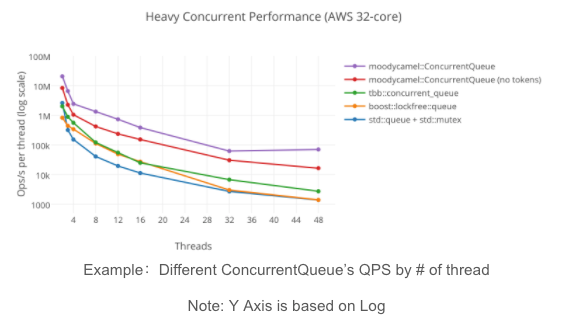
Heavy concurrent performance (AWS 32-core)
Source: A Fast General Purpose Lock-Free Queue for C++
In the Overcooked game, having more players doesn’t necessarily mean we can serve more dishes more easily. We need to have a discussion and form a good strategy before we start, so we will not step on each other’s toes. Otherwise, players could be competing for the same resource; for example, everyone is using the dishes but no one is washing the used ones. Or, since I am only responsible for cooking, I need to wait for the food to be chopped, but my upstream person is not doing it efficiently. This does not maximize utilization of the resources, and time is wasted on waiting.
As long as we can reach the maximum consumption of the bottleneck resource, we should minimize the number of concurrency threads. We also need to be aware of the hidden racing conditions. For example, if you perform a full table scan during a hash-join for a 1 GB table and each atomic task is 1 MB, there is a hidden racing condition. All the tasks need to access the same global hashmap during scanning. The granularity of accessing the hashmap is extremely small, which requires a large QPS and is likely to cause the system to race. It definitely creates a performance bottleneck during runtime.
Determine your parallelization strategies during the design phase
Just as we need to clearly communicate the strategy before clicking the play button in Overcooked, we need a strategy for parallelization during the design phase of our app. We will provide you with a cooking recipe to help you form a solid design for high throughput applications.
There are two principles for designing the parallelization strategy:
- Reduce the racing condition.
- Fully utilize the bottlenecked resource.
There are many parallelization strategies. Three common ones are:
- Global parallelization only.
- Global pipelining with local parallelization.
- Global parallelization with local pipelining.
The following table illustrates each strategy.
| Global parallelization only | Global parallelization + pipelining within each thread | Pipelining is the main process + parallelization on every step on the pipeline |
 |  |
The most common: global parallelization only
The most common strategy is global parallelization only. For example, if we have eight concurrent threads, one thread takes care of 1/8 of the task and just processes it alone. The threads do not necessarily have streaming or pipelining inside those threads’ execution. In the Overcooked game, this is like four different players working on a single order from beginning to end and not helping each other.
Global parallelization is the most common approach because it is the simplest to implement. When the performance requirement is not that high, it might be okay to run this way. But most of the time, this is not a good strategy for high throughput applications. This is mainly due to the lack of accurate control over the resource consumption by time, so there is no way for threads to collaborate on resource usage. The resource can’t be fully used: at one moment, the resource could be in peak usage in one thread, but idle in another. The threads don’t know one other’s status.
Global parallelization + pipelining
The second strategy uses global parallelization and applies pipelining within each thread. In the Overcooked game, this is like Players A and B working together on chopping, while Players C and D work together on cooking. Players A and B can collaborate: while one focuses on chopping, the other can start cooking.
One example of this implementation is found in ClickHouse, the Online Analytical Processing (OLAP) columnar database. To access disks, ClickHouse breaks the overall process into a number of threads for parallel computing and disk reading. Each thread works on a specific data range. Pipelining is applied during the disk reading step. If the reading is on a slow disk, the I/O is the bottleneck resource. On a fast disk, the CPU is the bottleneck resource. For either situation, since pipelining is applied, a tight bottleneck can have flat resource consumption. This is a good design for parallelization.
Pipelining without global parallelization
Another commonly used strategy uses pipelining as the main process without global parallelization, and it applies parallelization on every step on the pipeline. (Actually, this isn’t necessary; sometimes we could just use parallelization on the slowest step.) In the Overcooked game, the equivalent strategy is since cooking takes most of the time, players A, B, and C will all work on cooking, and player D will do the remaining work like chopping and washing dishes on their own.
This makes sense from a transaction perspective because it provides global data context when processing one step with all the resources in the system at one time. We also get better locality and better utilize the cache.
Last but not least, we can combine strategies based on our needs. As we discussed, many things could affect performance. Be sure to run benchmarks to determine the factors that affect your system’s performance.
Partitioning: a special kind of parallelization
Partitioning is a special kind of parallelization. Since different partitions do not share a task, we can consider partitioning using global parallelization only. With partitioning, we actually achieved a higher number of threads without the racing condition side effect.
However, partitioning has limitations. It requires that each partition must depend on one another. And the faster partition will need to wait for the slower part to finish. So the overall completion time of a task depends on the slowest shard to finish the work. The loss of waiting for a shard can be more than your expectation. The more partitions you have, the higher the loss associated with idle resources.
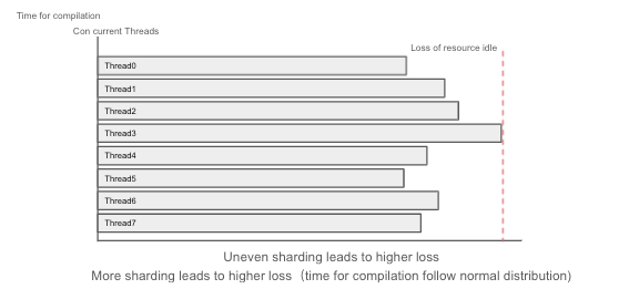
Uneven sharding leads to higher loss
More sharding leads to higher loss. Compilation time follows a normal distribution.
Summary
The digital transformation trend increases the workload and exposes challenges to system design. Adding resources to the processing system increases costs. Performance should be the result of design, not optimization. We can use streaming, pipelining, and parallelization to design our applications for better scheduling and fully utilize our bottleneck resource. This achieves a higher throughput on each node and increases the overall throughput of the system.
If you want to learn more about app development, feel free to contact us through Twitter or our Slack channel. You can also check our website for more solutions on how to supercharge your data-intensive applications.
Keep reading:
Using Streaming, Pipelining, and Parallelization to Build High Throughput Apps (Part I)
Building a Web Application with Spring Boot and TiDB
Using Retool and TiDB Cloud to Build a Real-Time Kanban in 30 Minutes
Spin up a database with 25 GiB free resources.


TiDB Cloud Dedicated
A fully-managed cloud DBaaS for predictable workloads
TiDB Cloud Starter
A fully-managed cloud DBaaS for auto-scaling workloads