TiDB Resource Control: Stable Workload Consolidation of Transactional Apps

Imagine you own data infrastructure at Super Sweet Tech, Inc (SST), a fictional company for the purpose of this story. Two big initiatives for the fiscal year fall to you. The first is to reduce costs. It’s not 2021 anymore, and the tech economy is tightening, along with its purses. The target is 20% reduction. Oof! The second is to reduce tickets related to data integrity. SST has heard enough from Twitter!

You and your group set out to identify problem areas, and you find two that seem to each touch on both initiatives. The first is datastore disparity, comprising 21 database types and 5,500 instances across them, all underpinning multiple APIs, microservices, and customer-facing applications. There are also downstream analytical stores, a lead into the second problem area. The analytics pipeline is a cost center and the main source of the data tickets, ultimately stemming from the mess of tooling involved and an enormous amount of tech debt that squeezes time for proper QA. 

A solution your group comes to is one that purports an impact on both initiatives. It would minimize the store disparity, pay down tech debt, and simplify CI/CD, documentation, and the skill sets required of your devs. Ultimately, these benefits would roll up to huge gains for the initiatives. 

The solution? Workload consolidation. If doable, this would mean combining online data from different applications and serving this data from one datastore or very few. Someone in your group brings you a blog about this very possibility.

This is that blog…

Introducing TiDB Resource Control

The latest stable release of TiDB (7.1) takes the idea of scaling transactional workloads an enormous step forward. TiDB, an extremely scalable distributed SQL database, guarantees consistency at these same scales. Even better, TiDB 7.1 introduces a new feature called Resource Control that really rounds out the story. It allows TiDB users to bring multiple applications together into a single backend. 

Consistency at scale is great for large online and data-intensive applications. But combining those applications into the same store? That’s spooky.

Bringing a data workload from somewhere else means introducing its CPU, memory, and disk consumption to that of the original application. App A…meet App B. Now play nice!

Resource Control (also referenced in this release blog) addresses the fears of online workload consolidation. It does so from the standpoint of compute CPU and storage I/O throughput (compute memory is addressed a different way) . Logical objects called Resource Groups control these items. These groups are logical buckets of cluster resources with an assigned priority. You can define separately both the bucket size and priority. You’ll learn more about them as we go.

Getting Started with TiDB Resource Control

Operators create these groups with a simple SQL command (shown later). Users (effectively, applications), sessions, and even single SQL statements can share the same bucket of resources when assigned to these groups. As you add more workloads to a group, it will maintain its constraints. If you add too many, those workloads may hit constraints and slow down. This is by design! The feature allows you more control over the stability of your high-traffic cluster in unpredictable scenarios. The choice between scaling to meet your applications’ needs and letting them underperform or fail is almost always an obvious one. Resource Control uses your requirements to maximize stability of your most important workloads.

Below is a concept diagram of the feature. It’s not important that you fully understand this image at this point. However, it may be worth coming back to as you learn more about these concepts later:

TiDB is a disaggregated architecture, such that compute and storage are separate (TiDB and TiKV, respectively, in the above diagram). Resource Control applies in both places. Given this, you should conceptualize the feature’s underlying mechanism as having two core functions: SQL flow control and storage priority-based scheduling. Flow control determines how requests are sent to storage in accordance with the availability of the resource quotas (RU_PER_SEC discussed later) in each Resource Group. Scheduling is the order of queuing (when queuing is necessary) for data access requests. This is determined by PRIORITY.

To make this hardline stability more flexible — while maintaining that stability — groups can also be defined as BURSTABLE. This means groups may use more resources than assigned, as long as they’re available. Making the most important workloads burstable means that even instant and unexpected increases in resource requirements can use more resources dynamically to keep response times within SLAs.

How It Looks

We can use an example to showcase what this might actually look like in the real world. To do this, I will show the creation of three Resource Groups: oltp, batch, and hr. The oltp workload represents our online and customer-facing application data. This is a critical and unpredictable workload and has strict latency SLAs that we will measure with tail latency (p99). The batch workload represents an analytics pipeline which is not customer-facing. This is still critical but less so, and will require less of the cluster. The hr workload represents a workload that is predictable and doesn’t have any SLAs associated with it.

Creating these groups happens in the SQL interface and would look like this:

CREATE RESOURCE GROUP oltp RU_PER_SEC=4000 BURSTABLE PRIORITY=HIGH;
CREATE RESOURCE GROUP batch RU_PER_SEC=400 BURSTABLE;
CREATE RESOURCE GROUP hr RU_PER_SEC=400;

The otlp group gets the highest quota because its members will be critical applications with periodically-high traffic. The batch group gets a smaller quota because it needs less and is less critical. However, time efficiency is a nice-to-have for the applications in this group. As a result, it is set to burstable to allow its applications to get greedy when space allows. The hr work, having the most leniency, gets the small quota with no ability to burst. This keeps it predictably “out of the way”.

Below is an example of how these groups might perform in a real-world scenario:

Notice that when the otlp workload needs a lot of resources, it gets them because it’s burstable and highest priority (top graph). While this workload eats its fill, its latency stays low and steady (bottom graph). As its traffic dies down throughout the day, the other burstable group can burst. Notice the batch workload’s change in latency as this happens. The hr group just does its thing.

So how does this work?

The Mechanism

Remember flow control and scheduling. To understand this, remember that TiDB is a disaggregated architecture. By that I mean compute (TiDB server), storage (TiKV), scheduling (Placement Driver) are physically decoupled:

That’s all you need to know about the architecture to understand the rest of this. Given that, I’ll jump right into the two previously mentioned core functions of the feature, flow control and priority-based scheduling.

Flow Control

The ultimate goals of Resource Control are to maintain expected consumption ratios of Resource Groups. Additionally, it ensures proper execution order of workloads with varying importance. To achieve the first goal, TiDB implements “flow control” to make and execute SQL requests. Resource Groups define and make decisions to send requests to storage (TiKV) with flow control.

The token bucket algorithm handles the flow control of data requests. In this case, “tokens” are Request Units (RUs) per second, or RUPS. The RUs are an abstraction of CPU milliseconds and disk I/O and can be read about in more detail here. RUPS of Resource Groups handle the rate at which the RU bucket backfills when requests in that group consume them.

As TiDB serves requests assigned to certain Resource Groups, both it and TiKV report information on the resources used by each request, which become RUs. The currently available RUs of the Resource Group subtract the RUs pertaining to the calculated request. They backfill at a rate commensurate with RUPS.

Priority-Based Scheduling

In accordance with the second goal of Resource Control, priority-based scheduling exists for two important reasons. The first is rather obviously to enforce order of execution for workloads of varying business priority. The second is to ensure that workloads of equal priority continue to get as close to their proportional amount of work done, even under resource constraints. While flow control aims to maintain this proportion, storage nodes must also own this because workload proportion can skew outside of the compute layer’s control (more on this later).

Priority-based scheduling is the mechanism by which TiKV puts data access requests from TiDB on an execution queue. This queue is a linked list of tasks in order of priority and then FIFO. The queue removes the tasks by a thread pool of concurrent threads extremely quickly. The tasks have a priority according to that of the request from a Resource Group. The head of the queue includes high-priority tasks, medium somewhere in the middle, and low priority tasks at the tail:

Given that Resource Control must ensure the storage layer is also treating Resource Groups according to their overall RU ratio, TiKV nodes must each be aware of global consumption rates of all Resource Groups.

Global Control

Without global control, prioritization of certain resource groups’ requests at each storage node may result in a skewing of the ratio. This is likely to happen if Resource Groups need uneven access to storage nodes and the nodes are not aware of what’s happening globally. But there’s good news!

While TiDB server’s flow control naturally addresses this via the globally-aware Placement Driver—from which it makes its requests for RUPS—TiKV nodes also address this their own way. 

To make sure groups continue to get their fair share of work globally, even in hotspot scenarios, TiKV nodes report real-time Resource Group usage as part of their response to the TiDB server’s request for data. This means all nodes receiving requests from those same TiDB server nodes are aware and can prioritize/deprioritize as necessary to maintain global proportions.

I think it would help to see examples of the two of these mechanisms working together. To illustrate this global awareness for ensuring ratios align with goals, I will ask you to engage your imagination once more in a few different scenarios. Each scenario has three applications assigned to Resource Groups, “rg1” , “rg2”, and “rg3”. For simplicity, each scenario uses a cluster with three storage nodes and we can know the theoretical max QPS (queries per second) for the cluster. Note: we’re using QPS as an abstraction of RU just to illustrate the final effect.

TiDB Resource Control Scenario 1

Groups rg1, rg2, and rg3 all have equal priority and the cluster can handle a theoretical max QPS of 4,000 (1,333 per node). The QPS needed for each group to maintain their apps’ SLAs is 1,000 (3,000 total). The below diagram illustrates how the Resource Groups’ workloads distribute, assuming the data they need access to evenly distributes across the nodes. Since priority is equal, I’ve left it out (it’s coming though):

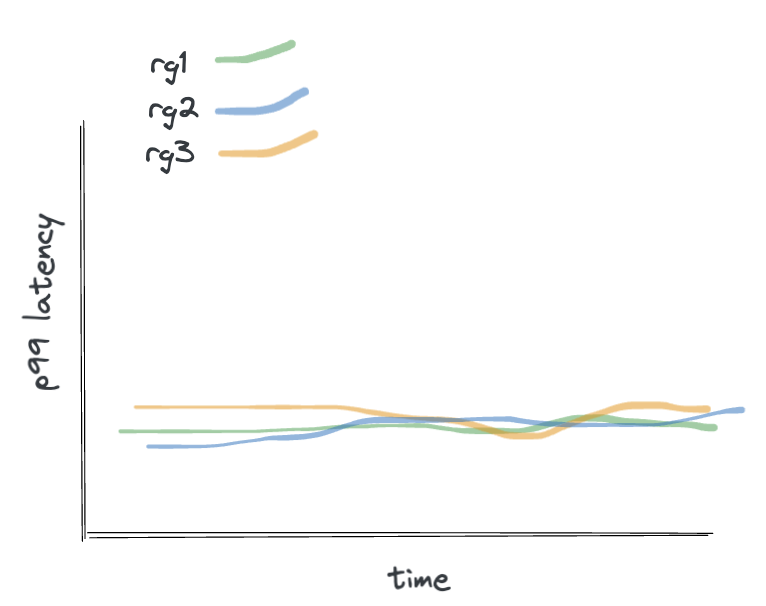
Since the available QPS of the cluster was enough for all groups and the priority of the groups were all the same, the workload distribution is complete and even, and the proportion is all 1:1:1. The fairness here will allow all applications assigned to the groups to maintain their SLAs, exemplified in the graph showing their steady latencies.

TiDB Resource Control Scenario 2

Now let’s say one workload assigned to rg2 makes rg2 require 3,000 QPS instead of 1,000. This means the total QPS required for the workloads exceeds the cluster’s max QPS. With an expected ratio of 1:3:1, resources constrain and some tasks will queue. As a result, we should get this:

Latencies for each group should rise as the nodes are now having to queue tasks due to resource saturation. However, even in this scenario, fairness is maintained and latencies are still comparable to one another. Also notice that, while the total QPS achieved by each Resource Group is under its requirement, the required ratio is maintained at 1:3:1.

TiDB Resource Control Scenario 3

Now we add PRIORITY. Let’s say rg2 gets a PRIORITY = HIGH while the other two get MEDIUM. Using the values from the previous scenario, the ratio may be 1:3:1 still but rg2’s priority will override that. Latencies of rg1 and rg3 may be affected as well:

In this scenario, every task sent to TiKV from rg2 is prioritized over those of rg1 and rg3. This is why we see the new 1:6:1 ratio; where rg2’s QPS requirements are satisfied and the other two groups fall short. Additionally, since rg2 tasks were cutting in line and it had higher throughput, the tasks for other groups had to wait longer than they did when queuing resources were available and queuing wasn’t required. This is by design!

In an ideal world, you would scale up your cluster as your workloads change in real time but…c’est la vie. What matters here is that the higher-priority, higher-throughput workload completed work on time and the cluster did worked on the other groups with the remaining time left.

TiDB Resource Control Scenario 4

Lastly, we’ll showcase the value of each TiKV node having that global awareness with a “hot spot” scenario.

An Example

All groups will have equal priority and QPS again, but this time each group requires 2,000 QPS. The ratio of workloads is 1:1:1 again but the resources are constrained and rg2 is now a “hot spot” workload. That means the keys it needs access to are more physically contiguous and located on the same storage node. Since all of rg2’s data is in TiKV 1, it can only use TiKV 1 to service its requests. This poses a potential problem for maintaining proportions across the cluster:

In this example, the “bad” outcome is where the resource consumption ratio (4:1:4) is askew from the target (1:1:1), and is what likely would have happened had TiKV nodes not been globally aware of Resource Group consumption. TiKV 1 would have naively tried to maintain proportions by using only its own scope to measure that. However, TiKV 1’s awareness that rg2 is getting no work on other nodes lets it prioritize those requests locally.

That’s right. Even though each group has an equal priority setting, on this specific node, rg2 gets higher priority so as to maintain global workload proportions. Since rg2’s workload is more than the node can handle, the node works on only this group, leaving other nodes to work on the other groups. Ultimately, you should scale this cluster, but in the meantime, proportions are kept according to plan. While tasks are being queued because of resource constraints, this mechanism ensures optimal prioritization cluster-wide.

Hopefully these example scenarios sufficiently showcase why priority-based scheduling as implemented really rounds out performance stability in a busy cluster. Combined with SQL flow control, separate workloads should resource-isolate from one another while remaining confident that data access requests execute with appropriate priority.

Conclusion

That wraps up the deep dive into the TiDB Resource Control feature. So what happened with our fictional company SST and its two big initiatives?

Well, it just so happens that this blog from a super sweet distributed database provider compelled them to POC the database. With this Resource Control feature, they found they were able to deploy a single cluster in each of their application regions that could scale to power all their online regional workloads. With TiDB Resource Control, each application with strict SLAs used the resources it needed to meet those SLAs. At the same time, they enabled users to run ad-hoc analytics directly on the raw source data without interfering with the production applications. This had the added benefit of making analytics available in online real-time.

TiDB Resource Control drastically mitigated their identified problem areas. For one, the skill sets needed to operate their backend shrank. While not immediate, most engineers responsible for backend infrastructure only needed to understand TiDB, made easier by the fact that it looks like MySQL to their applications. They were also able to reduce their CI/CD complexity, dev hours, and required documentation, which freed up time for engineers to focus on data quality and removed tech debt that prevented prioritizing outstanding bugs.

For more information on how to use TiDB Resource Control, please refer to the documentation.